Activity 8: Morphological Operations

Objective: To demonstrate the concepts of image dilation and erosion via a structuring element.

Tools: Scilab with SIP toolbox

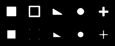
Procedure: We use an image set as shown below. The square is 50 by 50 pixels while the hollow square is 60 by 60 and 4 pixels in width. The traingle is 30 by 50 while the circle is 25 pixels in radius. On the other hand, the cross is 8 pixels wide and each arm is 50 pixels long.

ORIGINAL

We use the following structuring elements:

SE1=

1 1 1 1

1 1 1 1

1 1 1 1
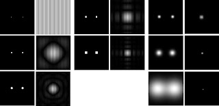
DILATION AND EROSION USING SE 1

SE2=

1 1 1 1

1 1 1 1

DILATION AND EROSION USING SE 2

SE3=

1 1

1 1

1 1

1 1

DILATION AND EROSION USING SE 3

SE4=

0 0 1 0 0

0 0 1 0 0

1 1 1 1 1

0 0 1 0 0

0 0 1 0 0

DILATION AND EROSION USING SE 4

We notice distinct changes in the images (which incidentally do not correspond to the predictions made previously). Using a square SE we simply see a transfromation of the structure either as an expansion of the lines in case of dilation and compression with erosion. For the non-symmetric elements( like the 2x4 and 4x2 ones), the expansion or contraction only applies to the elements parallel to the longitudinal axis of the SE. On the other hand, the cross SE yields transformations on both axes as well as the characteristic edge rounding of small SEs.

Acknowledgements: I would like to thank Mr. Cabello and Mr. Panganiban for their assistance.

Evaluation: Since the predictions do not match the result only a grade of 8 is seen as appropriate.

Activity 7:Enhancement in the Frequency Domain

Objectives: To demonstrate the concept of filtering in the frequency domain and how this affect the quality of images.

Tools: Scilab with SIP toolbox

Procedure: We begin by finding the FTs of pairs of apertures such as the ones we have below.

As with the previous activity, the FTs of the various patterns appear as a convolution of the paterns of a single aperture. It is also of note that the Gaussian FT is still a Gaussian but is tranformed in the frequency space. That is, a wider, more spread out Gaussian function has a narrower transform in the FT space.

The next set of examples illustrate the us of filtering in the Fourier space to cancel out certain undesirable components in the images.For example, the image of the moon below has a set of vertical lines which are very pronounced. Also it has some horizontal scan lines which may be an artifact of the mosaic process. In order to remove these, we implement the following steps:

1. Take the FT of the image.

2. Create a mask to remove certain components.

3. Shift (fftshift) the mask so that the lower order componenents are on the outer portions of the image.

4. Multiply the mask and the FT

5. Take the FT of the product. and normalize.

For this image we use a cross shaped filter to cancel out the periodic, cosinusoidal frequencies in the x and y direction. Note that the mask does not cover the DC component as this contains a lot of information about all the points on the object. Hence if it is removed we lose valuable information. The resulting filtered image is shown below the original. Note that the lines have been removed and the image is cleare. However since we inadvertently removed other useful components, the image has less contrast and detail in some parts than the original.

On the other hand, we a decidedly more difficult image with the next one which is a patch from a painting on stretched canvas. The task is to remove the weave pattern to enhance the actual image. For this we work directly with the FT of the image. The bright spots symmetric about either the x or y axis are the frequencies we want to dscard for these indicate periodic, cosinusoidal patterns in image space. Thus we place circular masks at the positions of these points. We see that when such a mask is used to filter the image, we get a weave free image. Also if we now take our mask and use the centers as the locations of bight spots, that is if we invert the mask, then take the FT, we come up with a weave pattern similar to what we removed from the original image.

For the last section, we attempt to enhance the ridges and lines on an image of a fingerprint. From the FT we discern that our region of interest is the band like structure centered about the DC component. We make a mask to leave only this and the DC component. We see that indeed we can recover the medium frequency components and enace the lines while removing most of the high order noise.

Evaluation: Since all the images were adequately enhanced using FT methods, a grade of 10 is applicable.

Acknowledgements: I would like to thank Misters. Garcia, Gubatan, Panganiban and Cabello for their helpful inputs.

Rating: Since all the results tally with what is expected and the images are well filtered, a score of 10 is warranted.

Activity 6: Properties of the 2D Fourier Transform

Objective: To increase familiarity with the various

Tools: Scilab with SIP toolbox.

Procedure:

1. Familiarization of FT of Different 2D Patterns.

Using the same routines as with the previous activity, we take the FTs of the following apertures:
This yields the following FT patterns:

The first two patterns are identical to the ones from the previous activity. The third image is from an annulus and if we compute the far-field diffraction pattern(which is the same as the FT) we see that the result is a difference between two orders of Bessel functions. Hence we see a set of missing orders or fringes. The fourth is essentially the same only now the functions are sinc functions in x and y. The fourth is the double slit pattern at far field. This can be thought of as coherent oscillators interfering with each other. This means that the upper and lower sections cancel each others contribution. This leaves the central strip hence we only see a pattern at the center of the strip. The last image represents two circular apertures, this results in a modulation of the phase from the other hole causing the interfernce fringes that are superposed on the circular diffraction fringes.

2. Anamorphic Property of the Fourier Transform

A. We take a 2-D Sinusoid with frequency f=4:

We then take the FT of this pattern which yields two points in the transform plane. This corresponds to the frequency of the input. We do this for two other frequencies,f=1 and f=15 to get the following images arranged in increasing f:

We see that as the frequency increases, the points move further from the center. This makes sense if we treat the points as the frequncies of the sine waves (which they are). Thus as the frequency is increased the points move away from the center.

Now if we add a constant bias, we essentially add a field with all the possible frequencies present. Hence from Fourier theory, the FT of this is a single point. We see this when we get the mesh() of the biased sine wave. For comparison, we place on the left a mesh plot of the FT of the same wave without a bias:

The spike at the center represents the frequency of the bias or what is known as the zero-order component. Note that this is of a greater intesity than the sine spikes. If in a real image this becomes an issue, it is possible to subtract the constant value from the input image. This would leave the two spikes represnting the sine. The position of the spikes corresponds directly to the frequency hence we can find the spatial frequency of the fringes in areal image. On the other hand, if the bias is not constantand is a low f sine, we can use the FTs and remove the lower frequency component. We can then take the inverse transform to leave us with the filtered sinusoidal wave.

If we rotate the sine waves like the ones below:

We get the following patterns, which are consistent with the previous result:

If we multiply two sines or any function with two frequencies, we get a superposition of the transforms of both. In this case we use a product of two sne functions:

Which has a transform like:

This corresponds with what we expected as we see two sets of spikes which individually look like the pattern for a simple sine function.

For the last part, if wee add this function to the rotated sines above, we get an image which looks like:

Which has a transform like:

All this essentially tells us that the 2D FT obeys the priciple of superposition.

Reference: AP 186 Activity 6 Manual

Evaluation: For the proper results, a grade of 10 is warranted.

Activity 5: Fourier Transform Model of Image Formation

Objective: To introduce the use of the Fourier Transform or FT as the standard model for imaging applications highlighting the varied uses of this method for image processing.

Tools: Scilab with SIP toolbox.

Procedure:The activity is divided into 5 parts each with its own focus.

1. Familiarization with the discrete FFT:
This section focuses on the use of the FFT as the mathematical equivalent of a lens. For this section we use two shapes, a circle and a square as our object and essentially image it with a lens of infinite aperture via the 2-D FFT function:

The corresponding FTs for these are as follows:

These image on the left represents the Airy disk of a point like image and the left image represnts the sinc(x)*sinc(y) function from a square aperture. This is how the patterns will appear on the transform plane on the back focal plane of a lens. Incidentally, these two images represent the far field or Fraunhofer diffraction pattern of the two aperture illuminated by a plane wave. When the FT of these images are taken we get the FT of the FT which are just the original images. On the other hand, if we use as our image a capital letter "A" as we have below:

We get a Fourier transform like the one we have below:
This indicates a center of symmetry even if the original image is only laterally symmetric. We also note that this patten may be thought of as a superposition of many point spread functions interfering with each other thus yielding this complex pattern. If we now take the FT of this image, we get an inverted "A" which can be thought of as the image of the object as seen through a lens system:

2. Convolution-Simulation of an Imaging Device.

The Convolution theorem essentially states that when the transform of two functions are multiplied it is equal to the transform of the product of the original functions. When this is translated into imaging, the image of an object ban be thought of as the convolution of the aperture function and the transfer function of the lens (or any other imaging system). In this case we use the the capital letters "VIP" in white against a blackbackground and a series of circular apertures simulating the aperture stop of the imaging lens. We take the FT of the aperture as imaged by a lens and then multiply it with the aperture which is in the transfrom plane. we then take the FT one more time to simulate another imaging lens.

We use the following apertures with increasing size.

The corresponding imaged convolutions are:

These correspond well to the fact that a larger aperture will produce a clearer image compared to a smaller aperture. At small apertures, the diffraction from the aperture actually limits the resolution of the imaging system.

3. Correlation-Template Matching

The section on correlation utilizes an image with certain text and a template letter. The correlatio is maximum when the section of the image matches completely with the template. This results in a large spot or spread function at the location of the match. In this case, we use the image on the left and then a template for the letter "A." The correlation is displayed on the right of these two:

The bright points indicate the regions of maximum correlation and these correspond clearly with the locations of the letter A in the image on the left.

4. Edge detection using convolution integral

In this last section we use the same concept as template matching to find the edges of an image pattern. This time we use matrices as our teplate instead of imges. Again we use the VIP image and find its edges using the following matrices:

A= -1 -1 -1

2 2 2

-1 -1 -1

B= -1 2 -1

-1 2 -1

-1 2 -1

and

C= -1 -1 -1

-1 8 -1

-1 -1 -1

With the following results:

Reference: AP 186 Activity 5 Manual

Evaluation: For the sheer amount of work expended as well as the proper results a grade of

10 is warranted.

Acknowledgements: I would like to thank the usual people for their assistance.

Activity 4:Enhancement by Histogram Manipulation

Objective: To manipulate images via their corresponding histogram and to enhance images by altering the gray levels as indicated by the histograms.

Tools: Scilab with SIP toolbox.

Procedure: The first order of business is to convert a colored image into grayscale or find a low contrast grayscale image. In this case we use an image of the M17 Nebula taken by the Hubble Space Telescope from the site:

http://www1.cs.columbia.edu/~johnc/ta_page/6998s07/

schedule/proj1/proj1.html

We then take the histogram of this, as in the previous activity, by finding and counting the number of pixels which have a specific grayscale value and plotting these against the actual values. This yields a histogram like this:

We then take another function related to the histogram

called the CDF. This is essentially the cumulative sum

of the histogrm at each grayscale value. This is found simply by using the cumsum() function in Scilab. The CDF of the image above looks like:

In order to enhance the image the idealized CDF for thi

s is a straight, increasing line. Thus after generating such a f

unction, we use projection to replace the grayscale values in the original image with the grayscale values of the y-axis equivalents. This effectively replaces the grayscale values which cause the CDF to deviate from the ideal. The net effect, at least in theory is an increase in the contrast between light and dark regions. However as shown by the new, enhanced image below, the contrast does not change too drastically.

But if we look at the histogram and the CDF of this new image, we see that the new CDF is already ideal:

Additionally, we present other examples of images enhanced using respectively: