LAST POST

THIS IN THEORY IS THE LAST POST IN THIS BLOG!

Activity 19: Restoration of Blurred Images

Objectives: To demonstrate the concept of motion blur and its restoration as well as basic noise filtering.

Tools: Scilab with SIP toolbox.

Procedure: We begin with an ordinary image with text written on it, in this case we use a grayscale image of the Apollo 13 Mission Patch with the words "Apollo XIII" and "Ex Luna Scientia."

We are in theory to simulate motion blur using the equation:

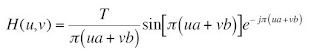
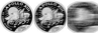
However, some difficulty was encountered in implementing this. As such the images were blurred using Photoshop, with varying distances of blur. After this, we add noise to the blurred image using the Gaussian image routine established in the previous activity, resulting in image like the one below:

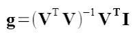
Then using the filtering method described in the activity, Weiner filtering, the original image is reconstructed using different parameters. The working equation is given as:

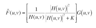
The reconstructed images for the middle sample above (with medium blur) follow:

Interestingly, the filtering routine seems to have worked even if the blurring functions used are of uncertain similarity. It appears that the blurring routine used in PS is similar to the routine we are to use here, but of course the correlation may be purely coincidental.

Evaluation: For the properly reconstructed images a grade of 10 is proper.

Acknowledgements: As usual Mr. Cabello and Panganiban have rendered invaluable assistance in this activity.

Activity 18: Noise Models and Basic Image Restoration

Objectives: To demonstrate basic noise modelling and the removal of noise from images using filters

Tools: Scilab with SIP toolbox, grayscale test and sample images

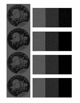
Procedure: We begin with a grayscale image of three gray levels from white to black. Simultaneously we use a real world image (in this case a grayscale image of the Apollo 13 Mission Patch) with more than three gray levels.

We model the different types of noise using mathematical models presented and add these noise matrices to both the test image and the real-world image. The following plate shows the images with different noise models added:

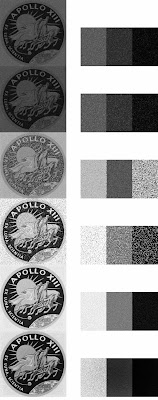
From top to bottom, the noise models are: Exponential, Gamma, Gaussian, Salt and Pepper, Uniform and Rayleigh noise. The added noise is then filtered on all the images using a variety of filters, described in the text (Arithmetic mean, Geometric mean, Harmonic mean and contraharmonic mean filters). The images above are processed using each of these filters and the results are shown below for each of the added noise types:

1. Exponential Noise

2. Gamma Noise

3. Gaussian Noise

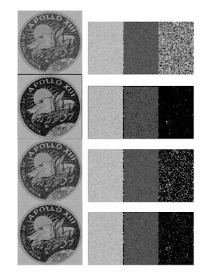4. Salt and Pepper Noise

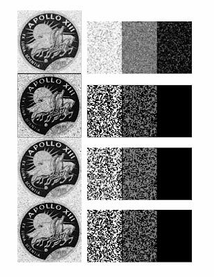
5. Uniform Noise

6. Rayleigh Noise

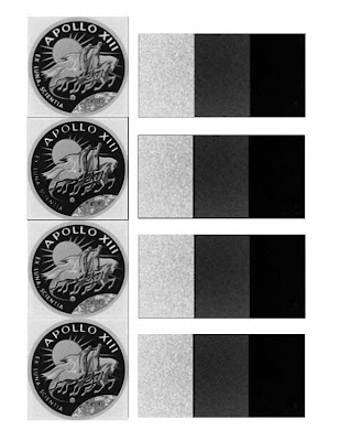
Evaluation: For correct noise models and filtering a grade of 10 is acceptable.

Acknowledgements: I would like to thank Mr. Panganiban for the invaluable assistance in this activity.

Activity 17: Photometric Stereo

Objectives: To reconstruct a three dimensional image using a set of 2-D images with different illumination positions.

Tools: Scilab with SIP.

Procedure: We start with four images of a spherical calibration target illuminated by a point source at these locations:

S1 = (0.085832, 0.17365, 0.98106)

S2 = (0.085832, -0.17365, 0.98106)

S3 = (0.17365, 0, 0.98481)

S4 = (0.16318, -0.34202, 0.92542)

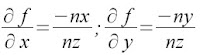
The positions vary by very small increments and hence the images do not appear to be any different to the eye. We find the surface normal vector to the points on the surface using the equation:

Where g is given by:

With V taken from the images. The slope with respect to z of each point in both x and y is given by:

The function f is fiven by the sum of the integrals of the partials in x and y. Numerically we use the cumulative sum fucntion to find these integrals and the resulting funtion is plotted in 3-D. The result is somehting like the plot below:

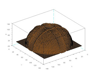
As we can see, the plot is hemispherical which is the result expected. It is of interest to examine the effect of varying the illumination shift on the accuracy of the reconstruction. It is also of note that this approach is from the stanpoint of intensity. That is, the changes in the illumination allow for the measurement of slope and shape. Another approach may involve the phase of the illuminating light which has been shown to yield better results in terms of reconstruction ability.

Evaluation: For the proper reconstruction of the shape, a grade of 10 is appropriate.

Acknowledgements: The assistance of Neil Cabello and Earl Panganiban is greatly appreciated.

Activity 16: Neural Networks

Objectives: To demonstrate the application of neural networks in pattern recognition

Tools: Scilab with SIP and ANN toolboxes

Procedure: As most of the details of the procedure are canned and those which are distinct are graphically repetitive, we shall go through what was done only in broad sweeping strokes. As mentioned, we used canned code for this, available through various channels. We first set a seed for consistency. We then create a training set of several values of two parameters, in this case as before, the area and red-color channel value of the intensities. For example we utilize the set:

y=

0.04 0.44

0.05 0.41

0.07 0.45

0.18 0.43

0.21 0.45

0.33 0.44

0.36 0.42

0.38 0.43

For this set, we classify this, in a manner similar to Boolean, as

[ 0 0 0 0 0 1 1 1]

That is to say, for our purposes, the last three sets, with the corresponding parameters are the ones to be classified under a certain heading and all the others effectively discarded.

Now we define a test set of object parameters we wish to classify:

x=

0.20 0.44

0.23 0.45

0.40 0.41

0.38 0.39

0.36 0.40

0.04 0.41

0.05 0.42

0.24 0.40

0.37 0.41

0.39 0.39

0.38 0.42

0.36 0.38

0.39 0.45

0.06 0.35

0.22 0.33

0.38 0.40

0.40 0.39

0.37 0.38

0.02 0.31

0.04 0.34

The output of the code, at a learning rate of 1 and with 1000 training cycles,rounded off to the nearest integer (1 or 0) is

[ 0 0 1 1 1 0 0 0 1 1 1 1 1 0 0 1 1 1 0 0]

Which is in exact agreement with what is expected. It is of note that when the learning rate is decreased, the pointwise accuracy of the network decreases. Additionally, the training cycle also has the same direct effect which agrees with intuitive understanding.

Evaluation: For proper classification a grade of 10 is appropriate.

Acknowledgement: As usual, Mr. earl Panganiban is of mention for his assistance.

Activity 15: Probabilistic Classification

Objectives: To apply Linear Discriminant Analysis to classify and sort objects from two distinct classes.

Tools: Scilab and data from Activity 14.

Procedure: The aim of the activity is to classify the objects in an

image into distinct groups in much the same way as the previous activity. Instead of using the distance method, we use linear discriminant analysis or LDA, the details of which can be found elsewhere. We utilize the same set of images from the previous activity, that of the coins.

As mentioned the data from the previous activity is used with same classification characteristics, that is area and color. Since we want to examine the usage of LDA on two classes of objects only, we sort our data set according to area and exclude the first ten values, as these correspond to one class of objects. This is to eliminate the need to mask one of the object test classes and redoing the image processing routines.

We then apply the LDA routine per the tutorial provided and plot in two axes, we get a figure similar to the previous activity. The crosses represent the loci of the objects in the image with respect to area and color.

Note the distinctive separation of the two classes with the lower set representing the lower denomination coins. Also of note is the better discrimination between the two classes compared to the previous activity. In the said procedure, the distinctions between two almost similar classes is unclear. In this case the deliniation is much clearer and hence it can be expected that this method will yield a better grouping and classification result.

Evaluation: For the proper classification of the objects a grade of 10 is appropriate.

Acknowledgements: The usual thanks to Neil Cabello and Earl Panganiban for the unfailing assistance.

Activity 14: Pattern Recognition

Objectives: To demonstrate the application of pattern recognition in describing a set or ensemble of objects in an image.

Tools: Scilab with SIP, an assembly of items with differnt shapes and sizes

Procedure: We begin by assembling a set of 30 coins representing our test objects. We use 10 each of .25, 1 and 5 Peso coins. The size of these coins increase with their denomination hence we can use that as one of our test parameters. Also the coins have different colors with the 25-centavo coin being bright copper, the one having a silver color and the 5 having a dull yellow-green tinge. We first take five of each coin and take a picture which we will use as our training set.

We then use a binarized copy of the image to find the areas of the coins using bwlabel. We do this for all the coins in the training set and group the similar values together. We then take the first five values and find the average which will then represent the average area of the one-peso coin. We do this for the next two sets of fives to get the areas for the other two coins. Then using the original image, we find the red-channel colors of each of the coins and in a similar manner find the average values. These two values, the area and the color represent our classifiation parameters which we then apply to a test set consisting of 10 coins of each denomination. arranged randomly within the field.

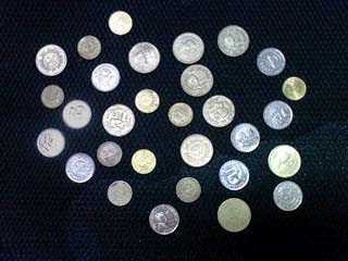
Using the same processing scheme as with the training set sans the averaging segment, we find our two classification parameters from the image and plot this with the x-axis being the area and the y-axis representing the color values of the red-channel.

Note that the cirlces represent the training parameters, that is the average color and area of each of the coins. We see a good clustering of the test points around the training values in the x-axis. This means that in terms of area, the coins in the test sample are quite distinguishable. However we still see a deviation from the ideal area which we can attribute to the changes in the area caused by the conversion from RGB to binary of the area measurement. Some of the coins shrink or expand depending on the lighting conditions and the thresholding value. Similarly in the y-axis we see a greater deviation from the average color values which again may be attributed to the lighting. Notice that the test and training images do not have exactly identical lighting conditions. As such some degree of deviation is expected. Of course this can be alleviated by employing more consistent lighting or in some cases, adding more features to test.

Evaluation: For the generally accpetable results, a grade of 10 is warranted.

Acknowledgements: The invaluable assitance of Mr. Earl Panganiban is greatly appreciated and is key to the completion of this excercise.

Activity 13: Correcting Geometric Distortion

Objectives: To demonstrate the process of correcting geometric distortions present in images.

Tools: Scilab with SIP.

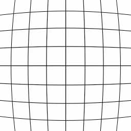
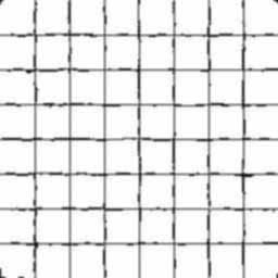
Procedure: In order to simplify the computation, we use a grid of horizontal and vertical lines with barrel distortion present like the one we have below:

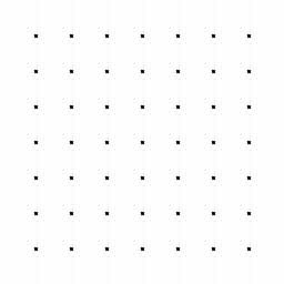
Using an idealized matrix of points, that is in the proper perpendicular vertex loci which is derived either using software or manually through the interface, we establish our reference grid. This is represented as a set of points occurring on the intersections of the lines.

Now using the least distorted part of the test grid image, we compute c1 through c8 using the following matrices:

Using linear algebra, the details of which we will omit as they are redundant, we get an expression for the coordinates of all the points of the image translated into the undistorted or proper frame:

This gives us the coordinates of the vertices in the correct frame. We use 2 interpolation methods to generate the points in between. We first use the bilinear interpolation which yields a grid like:

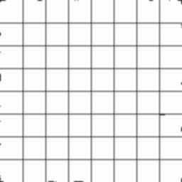
And then using the nearest neighbor interpolation we get:

As is consistent with theory, the bilinear method yields better results in terms of reconstructions.

Evaluation: For the properly reconstructed grid, a grade of 10 is justified.

Acknowledgements: As usual I thank Earl Panganiban and Gilbert Gubatan for their assistance.

Activity 11: Color Camera Processing

Objectives: To demonstrate the principle of color balancing in color cameras especially the post recording correction of improperly color balanced images.

Tools: Scilab with SIP toolbox

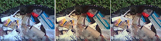
Procedure: We begin with several improperly color balanced images with several objects of different colors present. These have their color balance settings varied to show the effects of white balancing.

The right panel shows the result of the correction using the white patch algorithm. The images below show a drastically wrongly color balanced image corrected using both the white patch and grayworld algorithms

As can be seen from the images, the correction for both algorithms is generally acceptable. The white patch has more color fidelity especially in the red region while the grayworld is more uniform. However, for images which are dominated by a ceratin color, the gray world algorithm fails in that it generally overcorrects for a complimentary color. Hence, the white patch algorithm is a better all around method.

Evaluation: For the partially completed work, a grade of 7 is the highest appropriate score, as the algortihms were already implemented.

Activity 10: Preprocessing Text

Objectives: To apply image processing methods to isolate handwritten text from an imaged document.

Tools: Scilab with SIP toolbox

Procedure: We begin with a scanned image of text both handwritten and in type. Since the image is tilted, we make it upright using the mogrify() command in Scilab. For computing expediency we also resize the image to more managable dimensions.

We then crop a small portion of the image, with handwritten text to isolate then convert this to grayscale. Taking the FT as shown in the center image below allows us to see the components that we do not need, in this case the bright vertical line at the center corresponding to the horizontal lines on the image. Using a mask like the one on the right we can cancel this component out.

After eliminating the lines, we clean the images using morphological operators such as closing and opening and resizing . After cleaning, we use bwlabel() to label the text as we have in the middle frame below. Then we convert to binary to get just the hand written text.

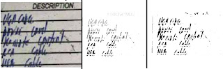
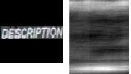
We also use image processing methods, in this case image correlation to find the occurences of a tempalte word, in this case "DESCRIPTION". The images below show the template word and the results of the correlation. The images appear to indicate very roughly the instances of occurence but are not as properly correlated as can be expected.

Evaluation: Since the text is not as clearly isolated and the correlation is not as proper, only 7 out of the possible 10 points is proper.

Acknowledgement: I would like to thank Mr. Cabello for constructive discussions.

Activity 9: Binary Operations

Objectives: To apply image processing techniques to the analysis of binary images and to do area measurement on such images

Tools: Scilab with SIP

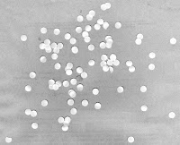
Procedure:We start with an image of a sheet of paper with holes randomly punched through, simulating cells in a microscope slide for example.

For computing expediency, cut up the image into nine panels of 256 by 256 pixels each. The images are read in grayscale and are binarized individually using im2bw with their own threshold values. This is done since there are areas of the original image which are darker or lighter than the rest of the image. As such each image needs a different threshold for converted to binary. After conversion, the "salt and pepper" noise on the converted images are removed by morphologically closing and opening the image. We have below the 9 binary images concatenated into a composite image:

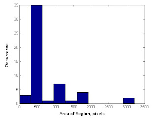
Using the bwlabel() function in Scilab, we label each individual hole and blob with a distinct integer. Then we use the find function to search for each of these values. We sum up all the values to find the area of each blob. Below, we have a histogram showing the number of occurences of a range of areas. We see that the most common areas are the small values corresponding to individual holes.

Evaluation: Since the results correlate closely with what is expected, a grade of 10 is proper.

Acknowledgements: I would like to thank Mr. Neil Cabello for his invaluable assistance.

Activity 8: Morphological Operations

Objective: To demonstrate the concepts of image dilation and erosion via a structuring element.

Tools: Scilab with SIP toolbox

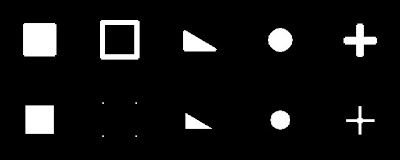
Procedure: We use an image set as shown below. The square is 50 by 50 pixels while the hollow square is 60 by 60 and 4 pixels in width. The traingle is 30 by 50 while the circle is 25 pixels in radius. On the other hand, the cross is 8 pixels wide and each arm is 50 pixels long.

ORIGINAL

We use the following structuring elements:

SE1=

1 1 1 1

1 1 1 1

1 1 1 1
DILATION AND EROSION USING SE 1

SE2=

1 1 1 1

1 1 1 1

DILATION AND EROSION USING SE 2

SE3=

1 1

1 1

1 1

1 1

DILATION AND EROSION USING SE 3

SE4=

0 0 1 0 0

0 0 1 0 0

1 1 1 1 1

0 0 1 0 0

0 0 1 0 0

DILATION AND EROSION USING SE 4

We notice distinct changes in the images (which incidentally do not correspond to the predictions made previously). Using a square SE we simply see a transfromation of the structure either as an expansion of the lines in case of dilation and compression with erosion. For the non-symmetric elements( like the 2x4 and 4x2 ones), the expansion or contraction only applies to the elements parallel to the longitudinal axis of the SE. On the other hand, the cross SE yields transformations on both axes as well as the characteristic edge rounding of small SEs.

Acknowledgements: I would like to thank Mr. Cabello and Mr. Panganiban for their assistance.

Evaluation: Since the predictions do not match the result only a grade of 8 is seen as appropriate.

Activity 7:Enhancement in the Frequency Domain

Objectives: To demonstrate the concept of filtering in the frequency domain and how this affect the quality of images.

Tools: Scilab with SIP toolbox

Procedure: We begin by finding the FTs of pairs of apertures such as the ones we have below.

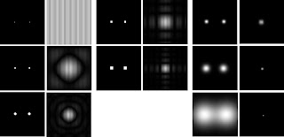
As with the previous activity, the FTs of the various patterns appear as a convolution of the paterns of a single aperture. It is also of note that the Gaussian FT is still a Gaussian but is tranformed in the frequency space. That is, a wider, more spread out Gaussian function has a narrower transform in the FT space.

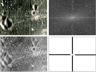
The next set of examples illustrate the us of filtering in the Fourier space to cancel out certain undesirable components in the images.For example, the image of the moon below has a set of vertical lines which are very pronounced. Also it has some horizontal scan lines which may be an artifact of the mosaic process. In order to remove these, we implement the following steps:

1. Take the FT of the image.

2. Create a mask to remove certain components.

3. Shift (fftshift) the mask so that the lower order componenents are on the outer portions of the image.

4. Multiply the mask and the FT

5. Take the FT of the product. and normalize.

For this image we use a cross shaped filter to cancel out the periodic, cosinusoidal frequencies in the x and y direction. Note that the mask does not cover the DC component as this contains a lot of information about all the points on the object. Hence if it is removed we lose valuable information. The resulting filtered image is shown below the original. Note that the lines have been removed and the image is cleare. However since we inadvertently removed other useful components, the image has less contrast and detail in some parts than the original.

On the other hand, we a decidedly more difficult image with the next one which is a patch from a painting on stretched canvas. The task is to remove the weave pattern to enhance the actual image. For this we work directly with the FT of the image. The bright spots symmetric about either the x or y axis are the frequencies we want to dscard for these indicate periodic, cosinusoidal patterns in image space. Thus we place circular masks at the positions of these points. We see that when such a mask is used to filter the image, we get a weave free image. Also if we now take our mask and use the centers as the locations of bight spots, that is if we invert the mask, then take the FT, we come up with a weave pattern similar to what we removed from the original image.

For the last section, we attempt to enhance the ridges and lines on an image of a fingerprint. From the FT we discern that our region of interest is the band like structure centered about the DC component. We make a mask to leave only this and the DC component. We see that indeed we can recover the medium frequency components and enace the lines while removing most of the high order noise.

Evaluation: Since all the images were adequately enhanced using FT methods, a grade of 10 is applicable.

Acknowledgements: I would like to thank Misters. Garcia, Gubatan, Panganiban and Cabello for their helpful inputs.

Rating: Since all the results tally with what is expected and the images are well filtered, a score of 10 is warranted.