Wednesday, September 30, 2009
Activity 19: Restoration of Blurred Images
Objectives: To demonstrate the concept of motion blur and its restoration as well as basic noise filtering.
Tools: Scilab with SIP toolbox.
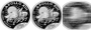
Procedure: We begin with an ordinary image with text written on it, in this case we use a grayscale image of the Apollo 13 Mission Patch with the words "Apollo XIII" and "Ex Luna Scientia."

We are in theory to simulate motion blur using the equation:
However, some difficulty was encountered in implementing this. As such the images were blurred using Photoshop, with varying distances of blur. After this, we add noise to the blurred image using the Gaussian image routine established in the previous activity, resulting in image like the one below:
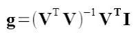
Then using the filtering method described in the activity, Weiner filtering, the original image is reconstructed using different parameters. The working equation is given as:
The reconstructed images for the middle sample above (with medium blur) follow:
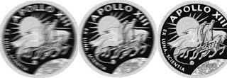
Interestingly, the filtering routine seems to have worked even if the blurring functions used are of uncertain similarity. It appears that the blurring routine used in PS is similar to the routine we are to use here, but of course the correlation may be purely coincidental.
Evaluation: For the properly reconstructed images a grade of 10 is proper.
Acknowledgements: As usual Mr. Cabello and Panganiban have rendered invaluable assistance in this activity.
Activity 18: Noise Models and Basic Image Restoration
Tools: Scilab with SIP toolbox, grayscale test and sample images
Procedure: We begin with a grayscale image of three gray levels from white to black. Simultaneously we use a real world image (in this case a grayscale image of the Apollo 13 Mission Patch) with more than three gray levels.


We model the different types of noise using mathematical models presented and add these noise matrices to both the test image and the real-world image. The following plate shows the images with different noise models added:
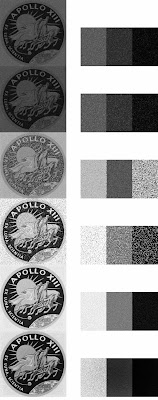
From top to bottom, the noise models are: Exponential, Gamma, Gaussian, Salt and Pepper, Uniform and Rayleigh noise. The added noise is then filtered on all the images using a variety of filters, described in the text (Arithmetic mean, Geometric mean, Harmonic mean and contraharmonic mean filters). The images above are processed using each of these filters and the results are shown below for each of the added noise types:
1. Exponential Noise
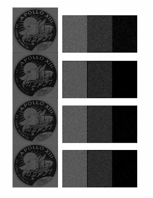
2. Gamma Noise

3. Gaussian Noise
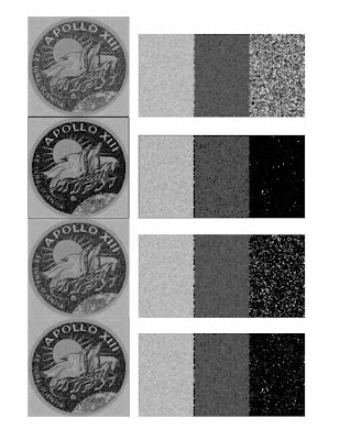 4. Salt and Pepper Noise
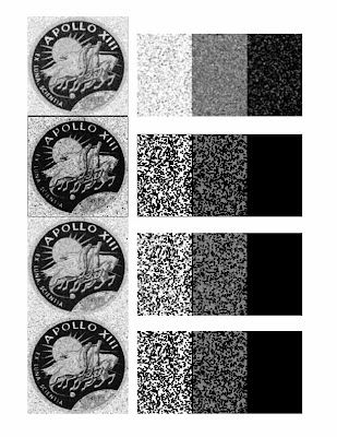
5. Uniform Noise
 6. Rayleigh Noise
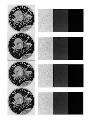
Evaluation: For correct noise models and filtering a grade of 10 is acceptable.
Acknowledgements: I would like to thank Mr. Panganiban for the invaluable assistance in this activity.
Wednesday, September 9, 2009
Activity 17: Photometric Stereo
Objectives: To reconstruct a three dimensional image using a set of 2-D images with different illumination positions.
Tools: Scilab with SIP.
Procedure: We start with four images of a spherical calibration target illuminated by a point source at these locations:
S1 = (0.085832, 0.17365, 0.98106)
S2 = (0.085832, -0.17365, 0.98106)
S3 = (0.17365, 0, 0.98481)
S4 = (0.16318, -0.34202, 0.92542)


The positions vary by very small increments and hence the images do not appear to be any different to the eye. We find the surface normal vector to the points on the surface using the equation:

Where g is given by:
With V taken from the images. The slope with respect to z of each point in both x and y is given by:
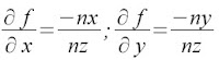
The function f is fiven by the sum of the integrals of the partials in x and y. Numerically we use the cumulative sum fucntion to find these integrals and the resulting funtion is plotted in 3-D. The result is somehting like the plot below:
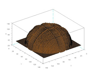
As we can see, the plot is hemispherical which is the result expected. It is of interest to examine the effect of varying the illumination shift on the accuracy of the reconstruction. It is also of note that this approach is from the stanpoint of intensity. That is, the changes in the illumination allow for the measurement of slope and shape. Another approach may involve the phase of the illuminating light which has been shown to yield better results in terms of reconstruction ability.
Evaluation: For the proper reconstruction of the shape, a grade of 10 is appropriate.
Acknowledgements: The assistance of Neil Cabello and Earl Panganiban is greatly appreciated.
Activity 16: Neural Networks
Objectives: To demonstrate the application of neural networks in pattern recognition
Tools: Scilab with SIP and ANN toolboxes
Procedure: As most of the details of the procedure are canned and those which are distinct are graphically repetitive, we shall go through what was done only in broad sweeping strokes. As mentioned, we used canned code for this, available through various channels. We first set a seed for consistency. We then create a training set of several values of two parameters, in this case as before, the area and red-color channel value of the intensities. For example we utilize the set:
y=
0.04 0.44
0.05 0.41
0.07 0.45
0.18 0.43
0.21 0.45
0.33 0.44
0.36 0.42
0.38 0.43
For this set, we classify this, in a manner similar to Boolean, as
[ 0 0 0 0 0 1 1 1]
That is to say, for our purposes, the last three sets, with the corresponding parameters are the ones to be classified under a certain heading and all the others effectively discarded.
Now we define a test set of object parameters we wish to classify:
x=
0.20 0.44
0.23 0.45
0.40 0.41
0.38 0.39
0.36 0.40
0.04 0.41
0.05 0.42
0.24 0.40
0.37 0.41
0.39 0.39
0.38 0.42
0.36 0.38
0.39 0.45
0.06 0.35
0.22 0.33
0.38 0.40
0.40 0.39
0.37 0.38
0.02 0.31
0.04 0.34
The output of the code, at a learning rate of 1 and with 1000 training cycles,rounded off to the nearest integer (1 or 0) is
[ 0 0 1 1 1 0 0 0 1 1 1 1 1 0 0 1 1 1 0 0]
Which is in exact agreement with what is expected. It is of note that when the learning rate is decreased, the pointwise accuracy of the network decreases. Additionally, the training cycle also has the same direct effect which agrees with intuitive understanding.
Evaluation: For proper classification a grade of 10 is appropriate.
Acknowledgement: As usual, Mr. earl Panganiban is of mention for his assistance.
Activity 15: Probabilistic Classification
Objectives: To apply Linear Discriminant Analysis to classify and sort objects from two distinct classes.
Tools: Scilab and data from Activity 14.
Procedure: The aim of the activity is to classify the objects in an
image into distinct groups in much the same way as the previous activity. Instead of using the distance method, we use linear discriminant analysis or LDA, the details of which can be found elsewhere. We utilize the same set of images from the previous activity, that of the coins.
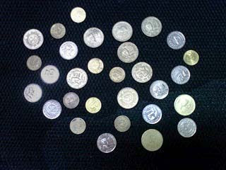
As mentioned the data from the previous activity is used with same classification characteristics, that is area and color. Since we want to examine the usage of LDA on two classes of objects only, we sort our data set according to area and exclude the first ten values, as these correspond to one class of objects. This is to eliminate the need to mask one of the object test classes and redoing the image processing routines.
We then apply the LDA routine per the tutorial provided and plot in two axes, we get a figure similar to the previous activity. The crosses represent the loci of the objects in the image with respect to area and color.

Note the distinctive separation of the two classes with the lower set representing the lower denomination coins. Also of note is the better discrimination between the two classes compared to the previous activity. In the said procedure, the distinctions between two almost similar classes is unclear. In this case the deliniation is much clearer and hence it can be expected that this method will yield a better grouping and classification result.
Evaluation: For the proper classification of the objects a grade of 10 is appropriate.
Acknowledgements: The usual thanks to Neil Cabello and Earl Panganiban for the unfailing assistance.
Subscribe to:
Posts (Atom)