Activity 14: Pattern Recognition

Objectives: To demonstrate the application of pattern recognition in describing a set or ensemble of objects in an image.

Tools: Scilab with SIP, an assembly of items with differnt shapes and sizes

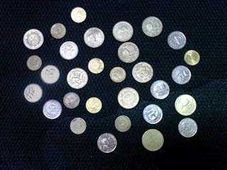
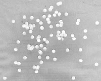
Procedure: We begin by assembling a set of 30 coins representing our test objects. We use 10 each of .25, 1 and 5 Peso coins. The size of these coins increase with their denomination hence we can use that as one of our test parameters. Also the coins have different colors with the 25-centavo coin being bright copper, the one having a silver color and the 5 having a dull yellow-green tinge. We first take five of each coin and take a picture which we will use as our training set.

We then use a binarized copy of the image to find the areas of the coins using bwlabel. We do this for all the coins in the training set and group the similar values together. We then take the first five values and find the average which will then represent the average area of the one-peso coin. We do this for the next two sets of fives to get the areas for the other two coins. Then using the original image, we find the red-channel colors of each of the coins and in a similar manner find the average values. These two values, the area and the color represent our classifiation parameters which we then apply to a test set consisting of 10 coins of each denomination. arranged randomly within the field.

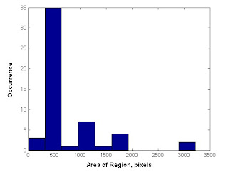
Using the same processing scheme as with the training set sans the averaging segment, we find our two classification parameters from the image and plot this with the x-axis being the area and the y-axis representing the color values of the red-channel.

Note that the cirlces represent the training parameters, that is the average color and area of each of the coins. We see a good clustering of the test points around the training values in the x-axis. This means that in terms of area, the coins in the test sample are quite distinguishable. However we still see a deviation from the ideal area which we can attribute to the changes in the area caused by the conversion from RGB to binary of the area measurement. Some of the coins shrink or expand depending on the lighting conditions and the thresholding value. Similarly in the y-axis we see a greater deviation from the average color values which again may be attributed to the lighting. Notice that the test and training images do not have exactly identical lighting conditions. As such some degree of deviation is expected. Of course this can be alleviated by employing more consistent lighting or in some cases, adding more features to test.

Evaluation: For the generally accpetable results, a grade of 10 is warranted.

Acknowledgements: The invaluable assitance of Mr. Earl Panganiban is greatly appreciated and is key to the completion of this excercise.

Activity 13: Correcting Geometric Distortion

Objectives: To demonstrate the process of correcting geometric distortions present in images.

Tools: Scilab with SIP.

Procedure: In order to simplify the computation, we use a grid of horizontal and vertical lines with barrel distortion present like the one we have below:

Using an idealized matrix of points, that is in the proper perpendicular vertex loci which is derived either using software or manually through the interface, we establish our reference grid. This is represented as a set of points occurring on the intersections of the lines.

Now using the least distorted part of the test grid image, we compute c1 through c8 using the following matrices:

Using linear algebra, the details of which we will omit as they are redundant, we get an expression for the coordinates of all the points of the image translated into the undistorted or proper frame:

This gives us the coordinates of the vertices in the correct frame. We use 2 interpolation methods to generate the points in between. We first use the bilinear interpolation which yields a grid like:

And then using the nearest neighbor interpolation we get:

As is consistent with theory, the bilinear method yields better results in terms of reconstructions.

Evaluation: For the properly reconstructed grid, a grade of 10 is justified.

Acknowledgements: As usual I thank Earl Panganiban and Gilbert Gubatan for their assistance.

Activity 11: Color Camera Processing

Objectives: To demonstrate the principle of color balancing in color cameras especially the post recording correction of improperly color balanced images.

Tools: Scilab with SIP toolbox

Procedure: We begin with several improperly color balanced images with several objects of different colors present. These have their color balance settings varied to show the effects of white balancing.

The right panel shows the result of the correction using the white patch algorithm. The images below show a drastically wrongly color balanced image corrected using both the white patch and grayworld algorithms

As can be seen from the images, the correction for both algorithms is generally acceptable. The white patch has more color fidelity especially in the red region while the grayworld is more uniform. However, for images which are dominated by a ceratin color, the gray world algorithm fails in that it generally overcorrects for a complimentary color. Hence, the white patch algorithm is a better all around method.

Evaluation: For the partially completed work, a grade of 7 is the highest appropriate score, as the algortihms were already implemented.

Activity 10: Preprocessing Text

Objectives: To apply image processing methods to isolate handwritten text from an imaged document.

Tools: Scilab with SIP toolbox

Procedure: We begin with a scanned image of text both handwritten and in type. Since the image is tilted, we make it upright using the mogrify() command in Scilab. For computing expediency we also resize the image to more managable dimensions.

We then crop a small portion of the image, with handwritten text to isolate then convert this to grayscale. Taking the FT as shown in the center image below allows us to see the components that we do not need, in this case the bright vertical line at the center corresponding to the horizontal lines on the image. Using a mask like the one on the right we can cancel this component out.

After eliminating the lines, we clean the images using morphological operators such as closing and opening and resizing . After cleaning, we use bwlabel() to label the text as we have in the middle frame below. Then we convert to binary to get just the hand written text.

We also use image processing methods, in this case image correlation to find the occurences of a tempalte word, in this case "DESCRIPTION". The images below show the template word and the results of the correlation. The images appear to indicate very roughly the instances of occurence but are not as properly correlated as can be expected.

Evaluation: Since the text is not as clearly isolated and the correlation is not as proper, only 7 out of the possible 10 points is proper.

Acknowledgement: I would like to thank Mr. Cabello for constructive discussions.

Activity 9: Binary Operations

Objectives: To apply image processing techniques to the analysis of binary images and to do area measurement on such images

Tools: Scilab with SIP

Procedure:We start with an image of a sheet of paper with holes randomly punched through, simulating cells in a microscope slide for example.

For computing expediency, cut up the image into nine panels of 256 by 256 pixels each. The images are read in grayscale and are binarized individually using im2bw with their own threshold values. This is done since there are areas of the original image which are darker or lighter than the rest of the image. As such each image needs a different threshold for converted to binary. After conversion, the "salt and pepper" noise on the converted images are removed by morphologically closing and opening the image. We have below the 9 binary images concatenated into a composite image:

Using the bwlabel() function in Scilab, we label each individual hole and blob with a distinct integer. Then we use the find function to search for each of these values. We sum up all the values to find the area of each blob. Below, we have a histogram showing the number of occurences of a range of areas. We see that the most common areas are the small values corresponding to individual holes.

Evaluation: Since the results correlate closely with what is expected, a grade of 10 is proper.

Acknowledgements: I would like to thank Mr. Neil Cabello for his invaluable assistance.